Wake losses remain the major source of uncertainty in energy production estimates (EPEs). And as we move toward multi-gigawatt clusters, larger turbines, and new wind development regions with unique weather conditions, that uncertainty is only decreasing.

Validating wake models is therefore critical, and it begins with measuring observed wake losses across a wind farm. Countless studies describe how to do this, yet nearly all report a single estimate of wake loss.

That has never sat right with me. “Observed wake loss” is not a fixed truth waiting to be measured. Rather it’s the outcome of dozens of analyst decisions. Which periods are filtered for downtime? How is spatial variability in the wind resource treated, especially in complex terrain? Which turbines are deemed “free stream”? Each choice can shift results, sometimes dramatically. Observed wake loss, therefore, is not a single measurement but a distribution of possibilities.

At Veer, we think it’s time to confront that complexity directly. In this post, we show how applying a Monte Carlo approach to calculating observed wake losses, where we sample from known uncertainties in the process, reveals a distribution of wake losses and our confidence in their values.

This work builds on earlier research by Eric Simley and colleagues at NREL, who also applied Monte Carlo methods to quantify uncertainty in observed wake loss estimates. We extend that concept further, incorporating new sources of uncertainty not previously considered.

So grab a coffee—this one’s a deep dive.

The Analyst’s Dilemma

On the surface, calculating farm-wide wake losses seems easy: just isolate free-stream from waked turbines and calculate the difference in their relative power outputs. In reality, however, measuring farm-wide wake losses involves a chain of methodological decisions, each capable of materially influencing the result. Below, we outline four of the most consequential analyst choices.

Filtering for Normal Production

In an ideal world, every turbine at a wind farm would be operating normally all the time, giving us a clean dataset of consistent production. In practice, outages and curtailments are inevitable, and wind farms rarely operate at full capacity. This poses a problem: if we filter out all timestamps with any downtime, we’re left with an inadequate sample size that is likely skewed by season or hour. If we don’t filter enough, we may let in too many downtime events, capture too many unrepresentative production periods and skew our wake loss calculations.

So how much missing data is acceptable? Should a timestep be discarded if 10% of turbines are offline? Is 5% to restrictive? Is 20% to permissive? There’s no universal standard, and each choice shifts the result. The “right” threshold likely depends on data quality and the performance characteristics of the site itself.

Spatial Heterogeneity

Wake losses are typically estimated by comparing “free stream” turbines with those operating in the wakes of others. This method works fine on flat, homogeneous terrain where free-stream production varies little between turbines. But in complex landscapes, natural variability in the wind field means turbines can produce differently even without wake effects. In some cases, your designated free-stream turbines might actually be the lowest producers on site!

To address this, it’s common to normalize observed turbine production relative to an expected power baseline derived from a wind map, such as a wind resource grid (WRG) file. Yet here, uncertainty creeps in again. WRG products vary widely in fidelity: some are driven by high-resolution mesoscale models (e.g., Vortex 100-m products), some from coarser mesoscale models and statistically downscaled (e.g., UL 50-m product) while others can be created from a single met mast timeseries measurement and linear extrapolations (e.g., UL’s 200-m product). Small discrepancies in the underlying Weibull parameters can meaningfully alter wake estimates. So the question becomes not just how to correct for spatial bias, but how reliable is the correction itself?

Free-Stream Turbine Designation

Determining which turbines qualify as “free stream” introduces another key uncertainty. Two parameters dominate: the upwind distance threshold and the angular width of the search window (see Figure 1). Wider, longer thresholds are conservative and help ensure wake-free flow conditions. Narrower, shorter thresholds are easier to satisfy but risk including turbines still influenced by wakes.

Obviously more conservative thresholds (large distance and large angular windows) are preferred. However, such thresholds are not always possible. In densely developed regions with many neighbouring wind farms, strict thresholds may yield no valid free-stream turbines for certain wind sectors, forcing analysts to relax criteria. Understanding the impact of those relaxed criteria is crucial.

Historical and Seasonal Representativeness

Even with careful filtering, spatial corrections, and free-stream identification, a final layer of uncertainty remains: time representativeness. Wake behaviour varies seasonally and diurnally, so a truly representative dataset should span at least one full year. But how typical is that year? How does an anomalously windy month or missing season bias the result? The available length and representativeness of the SCADA record can materially affect the robustness of wake loss estimates and can be explored in larger SCADA datasets.

In Summary

Taken together, these decisions highlight a deeper truth: wake validation is not a fixed measurement but a series of defensible choices, each carrying its own uncertainty. Filtering thresholds, spatial adjustments, free-stream designation, and temporal coverage all shape the losses we report. Three experienced analysts could apply equally rigorous methods to the same dataset and produce three different answers: all “correct,” yet all path-dependent.

That variability is the core challenge. Rather than chasing a single “right” value, we can embrace the distribution of possible outcomes and use statistical tools to quantify it.

Wind Farm Case Studies

To explore this idea in practice, we turn to a set of 11 onshore wind farms operated by one of our (very supportive) clients. For each site, we had access to SCADA data, permanent met masts, and high-resolution wind resource grids (WRGs) from multiple providers, providing a rich basis for both observed and modelled comparisons.

The farms span a diverse set of operating conditions (Table 1) from simple, open terrain to mountainous topographies and coastal regions with high spatial variability in the wind resource. We express this diversity in Table 1 through the “expected turbine power production range”, calculated as the difference in mean power output from the lowest- and highest-producing turbines. This metric is computed by taking Weibull coefficients from a WRG at each turbine location, sampling wind speeds from them 1 million times, and running those wind speeds through a site-specific power curve.

Table 1 shows a large range in spatial variability of expected power output. Site A, for example, has only a 3.9% expected power difference, while for Site K that difference balloons to 32.3%.

Data availability across the portfolio is robust: most sites have over five years of continuous SCADA records, with the remainder exceeding three years, ensuring strong temporal coverage for statistical sampling.

Table 1. Summary of Wind Farm Case Studies
Site	Expected Turbine Power Production Range (normalized)	Site Designation	Period of Record (years)
A	3.9%	Simple	>5
B	7.6%	Simple	3–5
C	8.7%	Simple	3–5
D	9.1%	Moderate	3–5
E	10.9%	Moderate	>5
F	11.0%	Moderate	>5
G	12.3%	Moderate	3–5
H	14.4%	Moderate	>5
I	18.0%	Complex	3–5
J	20.5%	Complex	>5
K	32.3%	Complex	>5

Methods

Here we describe the methods to get from SCADA data to distributions of observed wake loss estimates for the case study wind farms.

Data Cleaning and Gap-Filling

SCADA data for nacelle wind speed and active power are first screened to flag periods of abnormal turbine operation, such as curtailment, downtime, sensor errors, etc.. These flagged periods create data gaps that must be filled to ensure complete, comparable power series across all turbines for wake-loss estimation.

To address this, we use a correlation-driven imputation method designed to preserve both spatial and directional structure in the data. For each turbine:

Pairwise correlations are calculated among all turbine power series.
The most correlated peer turbines (correlation ≥ 0.8) are identified as predictors.
A Generalized Additive Model (GAM) is fitted to the valid data using two predictors:
- Power from the reference (most correlated) turbine, and
- Concurrent wind direction from the permanent met mast (PMM).

The model form is:

P_target = s(P_ref) + s(Wind Direction)

where s(⋅) denotes smooth spline functions.

The GAM captures both spatial coherence among turbines and directional dependence in performance. Missing power values are then replaced with model predictions, iterating through additional correlated turbines as needed until residual missing data fall below a small tolerance of 1%.

The result is a continuous, physically consistent power time series for every turbine, ready for accurate wake loss estimation and Monte Carlo sampling.

Wake Loss Calculation: General Approach

Estimating observed wake losses directly from 10-minute SCADA data is computationally intensive, especially when thousands of Monte Carlo realizations are required. Rather than operating timestep by timestep, we work at the sector-mean level, leveraging pre-aggregated relationships between turbines, the wind resource, and observed performance.

The process follows six main steps.

Define Directional Sectors: The number of wind direction sectors is taken from the site’s WRG, typically 16 (22.5° bins). Each sector is treated independently in subsequent calculations.
Compute Expected Power per Turbine and Sector: For each turbine and each sector, we compute the expected long-term mean power by sampling from the turbine’s Weibull wind-speed distribution.
- Weibull parameters (A, k) are extracted from the WRG at the turbine’s location.
- One million wind-speed samples are drawn from this distribution.
- Each sampled speed is converted to power via the site-specific turbine power curve.
- The mean of those simulated powers yields the turbine’s expected sectoral power.
Identify Free-Stream Turbines: For a given sector, we determine which turbines are likely to operate in clean, undisturbed flow. Using the turbine coordinate data, we identify all turbines that have no upwind neighbors within a specified distance limit (e.g., 5 km) and sector angular width ( ± 11.25°). These geometric parameters are later sampled across reasonable ranges in the Monte Carlo stage.
Calibrate Expected Power to Observed Free-Stream Performance: For each sector, we calculate the mean observed power of the free-stream turbines from the SCADA dataset and compare it with their expected power from the WRG. The mean ratio, ⍺, acts as a sector-specific calibration factor to correct the WRG bias. This correction is applied to expected power for all turbines in the sector.

 α = ( P̄_obs,FS ) / ( P̄_exp,FS )

 P_exp,adj = α · P_exp

Estimate Power Loss per Sector: Wake losses for each turbine are calculated as the difference between adjusted expected and observed power:

 ΔP = P_exp,adj − P_obs

The mean sectoral loss is then expressed as a fraction of the adjusted expectation:

 WL_sector = Σ ΔP / Σ P_exp,adj

Aggregate to Site-Level Loss: Finally, each sector’s wake loss is weighted by its frequency of occurrence, derived from the wind-direction histogram (bin frequencies) of the operational dataset:

 WL_site = Σ ( WL_sector · f_sector )

This mean-by-sector framework reduces data volume by several orders of magnitude, enabling efficient Monte Carlo sampling across thousands of analyst decision combinations.

Sampling Sources of Uncertainty

Observed wake losses are not defined by a single formula but by a web of interdependent analyst choices. To quantify that uncertainty, we represent each key methodological decision as a parameter that can be varied or resampled within a Monte Carlo framework. Each Monte Carlo realization samples across these parameters to produce an ensemble of plausible outcomes.

Four primary sources of uncertainty are considered:

Valid Power Threshold

Incomplete or invalid turbine data can bias observed power averages if handled inconsistently. For each timestep, we evaluate the percentage of turbines reporting valid power. We then apply Monte Carlo sampling thresholds varying between 5% to 20% in 1% increments to represent the uncertainty in how aggressively data should be filtered.

Free-Stream Geometry

Defining which turbines operate in “free-stream” flow introduces geometric uncertainty. Two parameters govern this classification:

Distance limit: Sample values between 3 km and 10 km upstream in 1-km increments.
Angular half-width: Sample values between 50% to 100% the WRG sector width (typically 22.5°) in 5% increments.

Temporal Representativeness

A single year of operation may not capture the long-term variability of wind speed, direction, or atmospheric stability.
To represent this uncertainty, we generate bootstrap “representative years” by resampling operational data in month–hour bins, preserving seasonal and diurnal structure while introducing stochastic variation. For each valid-power threshold, we generate 100 bootstrap years, yielding over 1,600 unique representative periods.

Wind Resource Grid (WRG) Source

WRG choice is not treated as a random Monte Carlo variable. Rather, we simply run the existing Monte Carlo framework defined above separately for each WRG source available at the wind farm site. In addition, we also perform the analysis without using any WRG or turbine power correction to examine the impact.

Results

Mean Wake Losses and Uncertainty

Figure 2 summarizes the mean observed wake losses and their associated uncertainties for all study sites, using the most representative wind resource grid (WRG) available at each location (either the Vortex 100-m, 16-sector product or the UL 50-m, 12-sector product, depending on data availability).

**Figure 2: Long-term wake losses with uncertainty intervals defined as the standard deviation of Monte Carlo sampling results.**

For each site, the mean wake loss is the Monte Carlo average, and the uncertainty is defined as the standard deviation of all wake-loss samples.

To examine how terrain influences results, sites are grouped into simple, moderate, and complex categories based on topography and flow conditions. The results show:

Wide variability across terrain types: Wake losses span a broad range, from just over 5% to nearly 14%, highlighting the diverse layouts, terrains, and weather across the sites.
No consistent link between complexity and uncertainty: All complexity classes include both high- and low-uncertainty sites, suggesting that site-specific factors like layout geometry, dominant wind sectors, and atmospheric stability play a larger role than wind spatial variability classification alone.

Sources of Uncertainty

To assess how different analyst choices influence observed wake-loss estimates, we performed a variance decomposition of the Monte Carlo results. Each uncertainty source was isolated in turn by holding all other parameters constant and re-running the Monte Carlo sampling. The standard deviation of wake-loss outcomes from each run was taken as that category’s standalone uncertainty, and each value was then normalized against the total uncertainty from the full-sampling case to compute percentage contributions.

This approach assumes independence among factors, so interaction effects are ignored, but it provides a clear, first-order view of which decisions most strongly drive uncertainty.

**Figure 3: Source contributions to total wake loss uncertainty**

In Figure 3, we show for each wind farm the contribution of each uncertainty category to total uncertainty. Key insights include:

Free-stream geometry dominates: Upstream distance and angular width account for the largest share of total variance across nearly all sites. This highlights how strongly wake-loss estimates depend on how “free stream” is defined.
Temporal representativeness has minimal impact: The choice of representative year contributes less than 15% of total variance, suggesting that wake-loss estimates are relatively stable across different annual conditions.
Data-quality thresholds matter at some sites: The valid power threshold generally contributes moderately. One exception is Site D, where this factor explains more than 60% of total uncertainty—higher than any other category observed.

To further explore these sensitivities, we examine how wake loss estimates trend at the different wind farms in response to variations in these core uncertainty parameters.

Figure 4 shows how wake losses vary with the valid power threshold. Across most wind farms, this effect is small, typically within ±0.4% of the baseline (5% threshold) wake loss. However, three sites exhibit a clear downward trend: wake losses decrease by up to 2.5 percentage points as the threshold is relaxed from 5% to 20%. This likely occurs because including more flagged periods introduces partial downtime events, when many turbines are curtailed or inactive, leading to physically weaker wakes across the site. The result is an artificial reduction in apparent wake losses.

While plausible, this behaviour underscores that data completeness can bias wake estimates if not carefully controlled. Further analysis—particularly cross-checking flagged intervals with downtime logs—would help confirm whether these trends reflect real flow physics or artifacts of missing data.

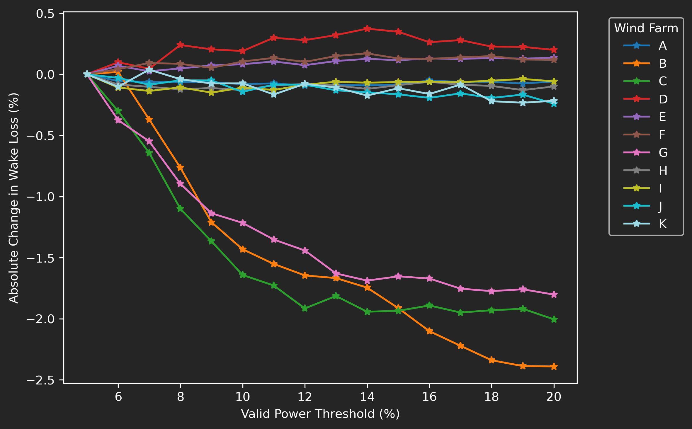
**Figure 4: Sensitivity of observed wake losses to changes in valid-power threshold, normalized to results at a 5% threshold.**

Figure 5 shows how estimated wake losses vary with the upwind search distance used to identify free-stream turbines, measured relative to a 3 km baseline.

Across nearly all sites, increasing the upwind distance leads to higher estimated wake losses. The magnitude of change differs by site, but the trend is consistent: as the search window extends, we gain greater confidence that the designated turbines operate in undisturbed flow. This increases the reference power level, which in turn amplifies the contrast between waked and unwaked turbines.

At shorter distances (e.g., 3 km), turbines classified as “free stream” may still experience residual wake effects, narrowing the observed difference and underestimating wake losses.

In principle, longer distance thresholds should yield more accurate results. However, such wide search windows are not always practical. In densely developed regions or multi-project clusters, neighbouring wind farms often limit the available upwind space, forcing the adoption of shorter thresholds and acceptance of a small downward bias in observed wake losses.

**Figure 5: Sensitivity of observed wake losses to changes in free-stream distance threshold, normalized to results at a 3-km threshold.**

Figure 6 explores how the width of the angular search window affects estimated wake losses. For each site, results are shown relative to a fixed 22.5° sector width baseline.

In most cases, wider search windows lead to higher wake-loss estimates. This trend follows expectations: expanding the angular window applies a more conservative free-stream definition, ensuring that selected turbines are well outside potential wake influence. Narrower windows, while including more candidate turbines, are more susceptible to contamination from meandering or partially aligned wakes, which can reduce apparent free-stream power and lower the calculated wake-loss magnitude.

One site departs from this pattern, showing a decline in wake loss as the angular window widens. Further analysis is planned to confirm the cause.

Note that not all sites extend to the maximum half-width of roughly 45°. In several projects, stricter thresholds eliminate free-stream candidates altogether in certain sectors, particularly at tightly spaced sites or where nearby wind farms constrain the available upwind area. These cases illustrate the practical trade-off between geometric rigor and data availability in wake validation.

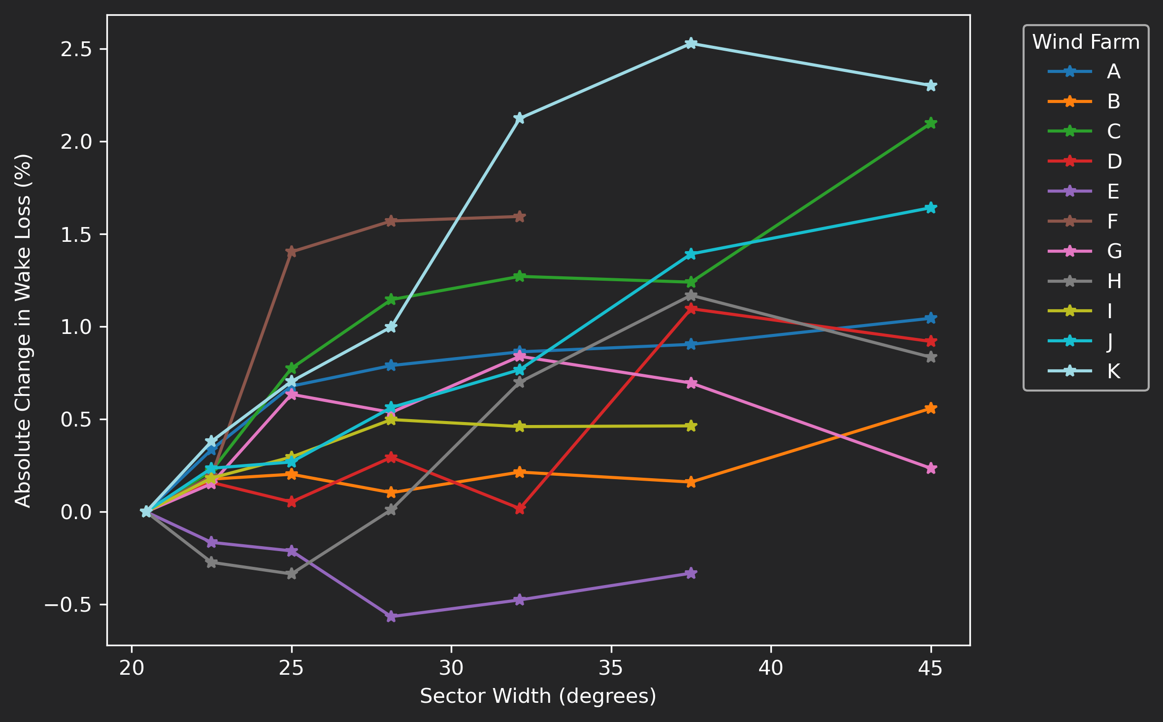
**Figure 6: Sensitivity of observed wake losses to changes in free-stream sector width threshold, normalized to results at a 22.5° threshold.**

Figure 7 compares estimated wake losses across different wind resource grid (WRG) products, including the use of no WRG, to assess how sensitive results are to the underlying wind resource model. We report results from all available WRG sources, typically one to three depending on the site.

Results show substantial variation and clear sensitivity to WRG choice. In simple terrain sites, such as Wind Farm A, differences between WRGs are small—often less than one percentage point. This consistency is expected where wind flow is uniform and turbine-to-turbine variation in expected power is minimal.

At complex sites, the influence of WRG selection becomes much stronger. As spatial gradients in wind exposure increase, the accuracy of each WRG’s local representation grows critical. At the most complex site, estimated wake losses ranged from roughly 7% using the WRG correction to –4 % when no WRG was applied, the latter implying “negative” wake losses and underscoring the pitfalls of uncorrected comparisons in heterogeneous flow fields.

These results emphasize the importance of using high-quality WRGs when estimating wake losses in complex environments. While this dataset is not broad enough to compare specific WRG providers, the trend is clear: as terrain complexity increases, so does the dependence of accurate wake estimation on the fidelity of the WRG.

**Figure 7: Sensitivity of observed wake losses to different WRG products used in the calculation.**

Finally, Figure 8 quantifies how sensitive wake-loss estimates are to the choice of WRG by comparing the standard deviation of wake losses across WRG products for each site against the maximum–minimum difference in expected turbine power derived from the primary WRG.

The relationship is clear and consistent: sites with greater turbine-to-turbine variation in expected power also show higher sensitivity of wake losses to WRG choice. At sites with nearly uniform flow, different WRGs yield nearly identical results. In contrast, as spatial variability increases, the same wake-loss calculation becomes increasingly dependent on how each WRG resolves local wind-speed gradients.

This finding reinforces a key pattern: WRG fidelity matters most in complex terrain. When spatial variability in wind resource is high, the representation of microscale flow patterns can shift estimated wake losses by several percentage points, enough to alter performance assessments and financial projections. Ensuring that WRG products accurately capture these gradients is therefore essential for credible wake validation.

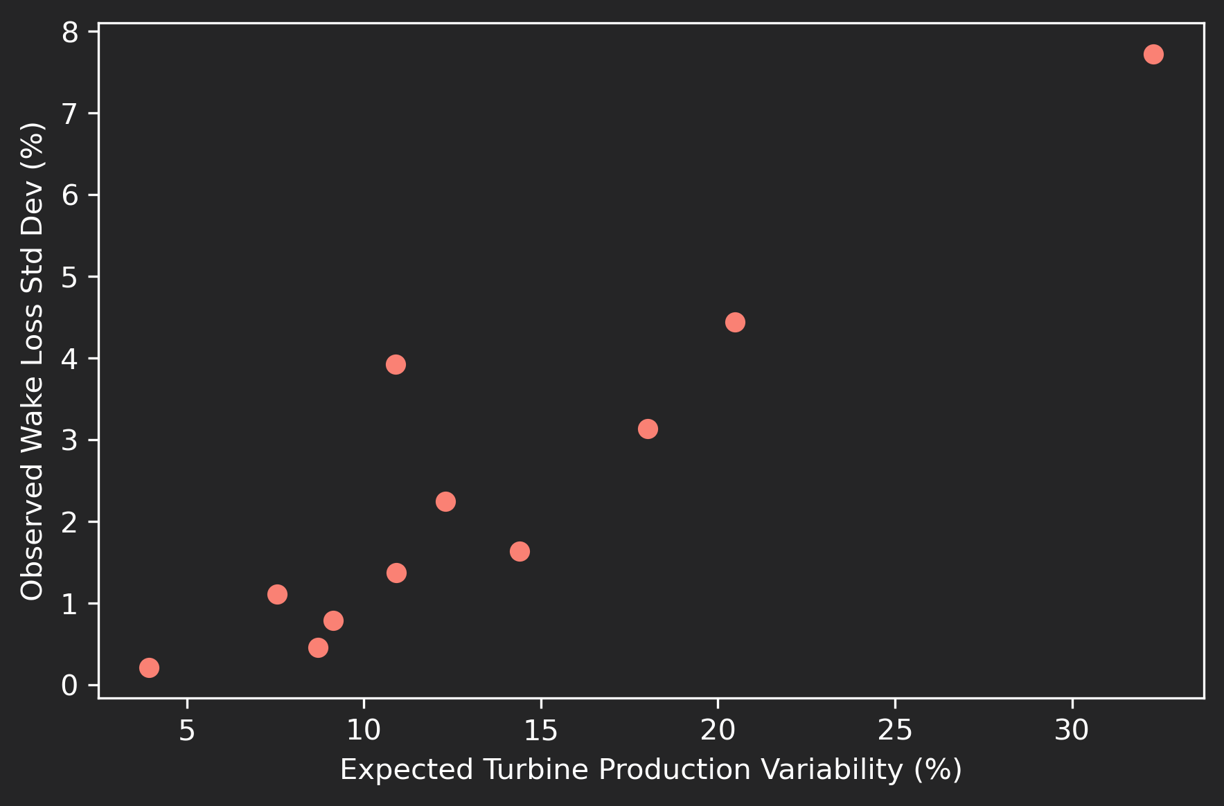
**Figure 7: Relationship between spatial variability in power output across site and sensitivity of observed wake losses to different WRG products.**

Conclusions

This study provides abroad exploration of how methodological uncertainty shapes estimates of observed wake losses at operating wind farms. By reframing observed wake loss calculation as a Monte Carlo sampling problem, we capture the full spread of results that naturally arises from different but reasonable analyst decisions. The goal was not to perfect the method, but to map the landscape of uncertainty and identify where refinements are most needed.

Several clear patterns emerge. The geometric parameters used to define free-stream turbines—upwind distance and angular search width—remain the largest sources of uncertainty. These are also the most constrained in practice: many wind farms simply lack sufficient upwind space to isolate clean flow, especially in regions with dense development or neighbouring projects. Shorter search windows inevitably bias results toward lower wake losses, yet expanding them is often impossible.

This raises a key question for the industry: how should we handle sites where true free-stream conditions no longer exist? Incorporating modelled external wake effects might seem like an answer, but it risks circularity: i.e., using a wake model to validate wake models. Still, without some representation of neighbouring influence, it becomes difficult to produce reliable site-level wake estimates in increasingly crowded landscapes.

The analysis also shows that WRG fidelity is critical in complex terrain, while temporal representativeness plays a smaller role than expected. Together, these findings suggest that future work should focus on three fronts:

Developing consistent approaches for handling proximity to neighbouring wind farms
Improving WRG accuracy in complex terrain
Extending the Monte Carlo framework to include cross-category interactions among uncertainties

This was an intentionally coarse first pass, leaving open questions and a few surprises still to unpack. Yet one message stands firm: there is no single observed wake loss for a wind farm. What we see instead is a distribution of outcomes, largely shaped by the analyst’s choices. Recognizing and quantifying that variability is the path to more honest, transparent wake validation.

There Is No Single “Observed Wake Loss”